Linear Regression Algorithm (線形回帰) [ 機械学習 ]

2014-04-08 17:07:00 +0900

Linear Regression は機械学習の中でも、歴史があり広く使われているアルゴリズムです。Perceptron アルゴリズムのようにアウトプットが +1 か -1 のような決定的なものではなく、実際の数字を取ることができます。クレジットカード審査の例で言えば、カード発行の許可・不許可という結果だけでなく、許可された場合にカードの限度額までアウトプットできます。しかし、Linear という名前が暗示しているように、基本的にデータは Perceptron と同じように直線で分類されることができなければなりません。

Linear Regression Algorithm

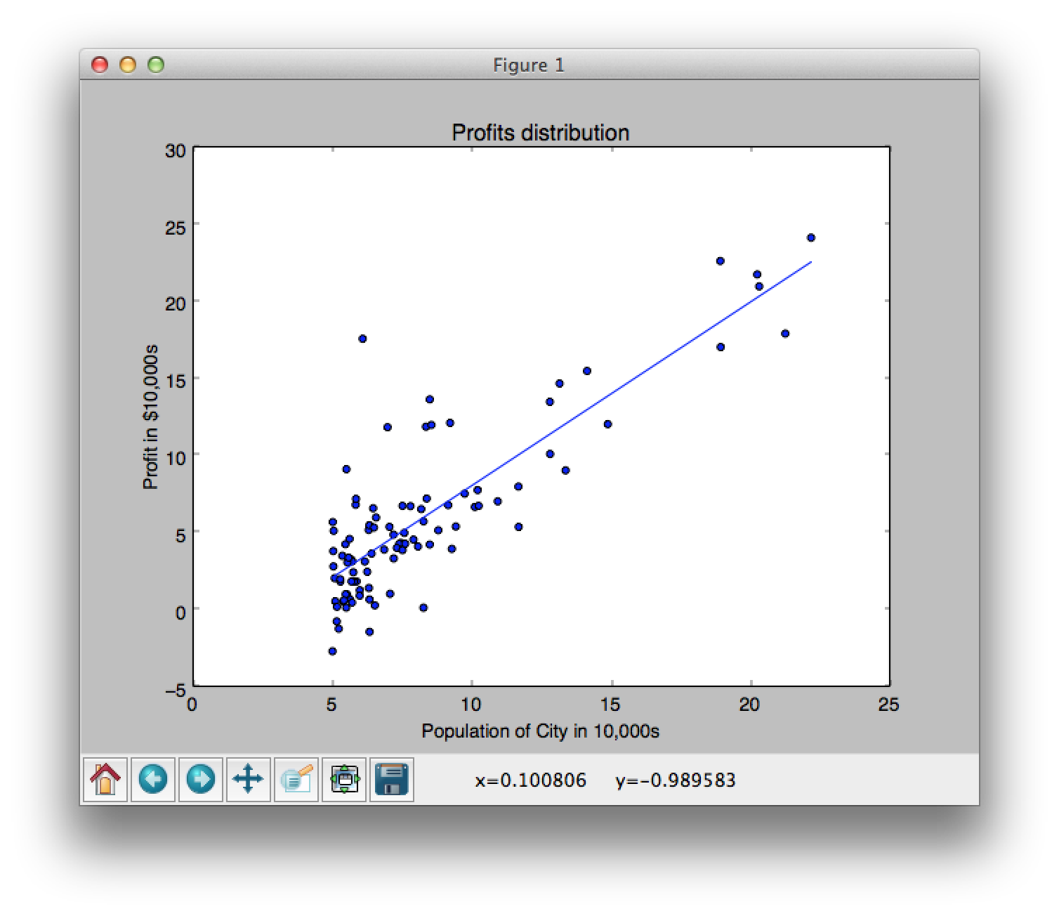
Linear Regression の一番の目標は、エラー率が最小化された結果を返すことです。図1の赤い線は実際のデータと予想された結果との差（エラー）を表しています。これが最小化されていれば、良い結果ということです。

このエラーを計算する方程式は、

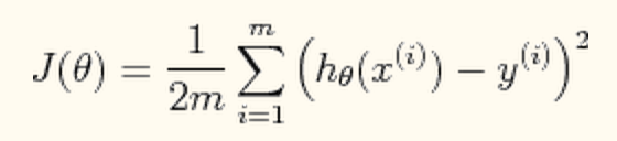
です。この J(theta) がエラー。m はサンプル数。x(i) がトレーニングデータ。y(i) がトレーニングデータの正確な結果（ターゲット関数の返り値）。h(theta)が仮説です。h(theta) は、

となります。x （インプット）と h のドット積です。

エラーを最小化するように theta を調整することが、今回の目標です。今回は、Gradient descent というアルゴリズムを使用します。

まず、theta を全て 0 に初期化します。そして、予め決められた回数分、ループを回してこの theta を最適化していきます。毎度、上記の式の通り、theta がアップデートされます。コードの中で、theta の値をアップデートし続けることで、J(theta) (エラー) の値がどんどん小さくなっていきます。J(theta)の値を print 等すれば、イメージがつかめると思います。

Code

Python で実装したコードがこちらです。このブログの作者が実装したものです。解説も分かりやすくとても参考になりました。大きな流れとしては、theta (仮説) を 0 に初期化して、その際の J(theta) （エラー率）を表示します。そして、gradient_descent 関数を呼び出し、実際の学習をし、結果を表示するという感じです。このコードは、ある会社の経営者が、新しいお店を出店したいという時に、現在出店されているお店の売上とその町の人口を使って、予想するというシンプルなものです。より洗練された変数の数が増えたケースもこのブログ記事には、解説されています。

# http://aimotion.blogspot.com/2011/10/machine-learning-with-python-linear.html
 
from numpy import loadtxt, zeros, ones, array, linspace, logspace
from pylab import scatter, show, title, xlabel, ylabel, plot, contour
  
#Evaluate the linear regression
def compute_cost(X, y, theta, isPrint=False):
    '''
    Compute cost for linear regression
    '''
    #Number of training samples
    m = y.size
  
    predictions = X.dot(theta).flatten()
  
    sqErrors = (predictions - y) ** 2
  
    J = (1.0 / (2 * m)) * sqErrors.sum()
 
    return J
  
  
def gradient_descent(X, y, theta, alpha, num_iters):
    '''
    Performs gradient descent to learn theta
    by taking num_items gradient steps with learning
    rate alpha
    '''
    m = y.size
    J_history = zeros(shape=(num_iters, 1))
  
    for i in range(num_iters):
  
        predictions = X.dot(theta).flatten()
  
        errors_x1 = (predictions - y) * X[:, 0] # X[:, 0] is all 1s
        errors_x2 = (predictions - y) * X[:, 1]
  
        # batch gradient
        theta[0][0] = theta[0][0] - alpha * (1.0 / m) * errors_x1.sum()
        theta[1][0] = theta[1][0] - alpha * (1.0 / m) * errors_x2.sum()
  
        J_history[i, 0] = compute_cost(X, y, theta, isPrint=True)
  
    return theta, J_history
  
  
#Load the dataset
data = loadtxt('ex1data1.txt', delimiter=',')
 
#Plot the data
scatter(data[:, 0], data[:, 1], marker='o', c='b')
title('Profits distribution')
xlabel('Population of City in 10,000s')
ylabel('Profit in $10,000s')
# show()
  
X = data[:, 0]
y = data[:, 1]
  
#number of training samples
m = y.size
  
#Add a column of ones to X (interception data)
it = ones(shape=(m, 2))
it[:, 1] = X
  
#Initialize theta parameters
theta = zeros(shape=(2, 1)) # [[0.][0.]]
  
#Some gradient descent settings
iterations = 3000
alpha = 0.01
  
#compute and display initial cost
print compute_cost(it, y, theta, isPrint=True) # 32.0727338775
  
theta, J_history = gradient_descent(it, y, theta, alpha, iterations)
  
print 'theta is', theta
#Predict values for population sizes of 35,000 and 70,000
predict1 = array([1, 3.5]).dot(theta).flatten()
print 'For population = 35,000, we predict a profit of %f' % (predict1 * 10000)
predict2 = array([1, 7.0]).dot(theta).flatten()
print 'For population = 70,000, we predict a profit of %f' % (predict2 * 10000)
  
#Plot the results
result = it.dot(theta).flatten()
plot(data[:, 0], result)
show()

参考

http://aimotion.blogspot.com/2011/10/machine-learning-with-python-linear.html
http://openclassroom.stanford.edu/MainFolder/DocumentPage.php?course=MachineLearning&doc=exercises/ex2/ex2.html

Category

Archive